Research Background

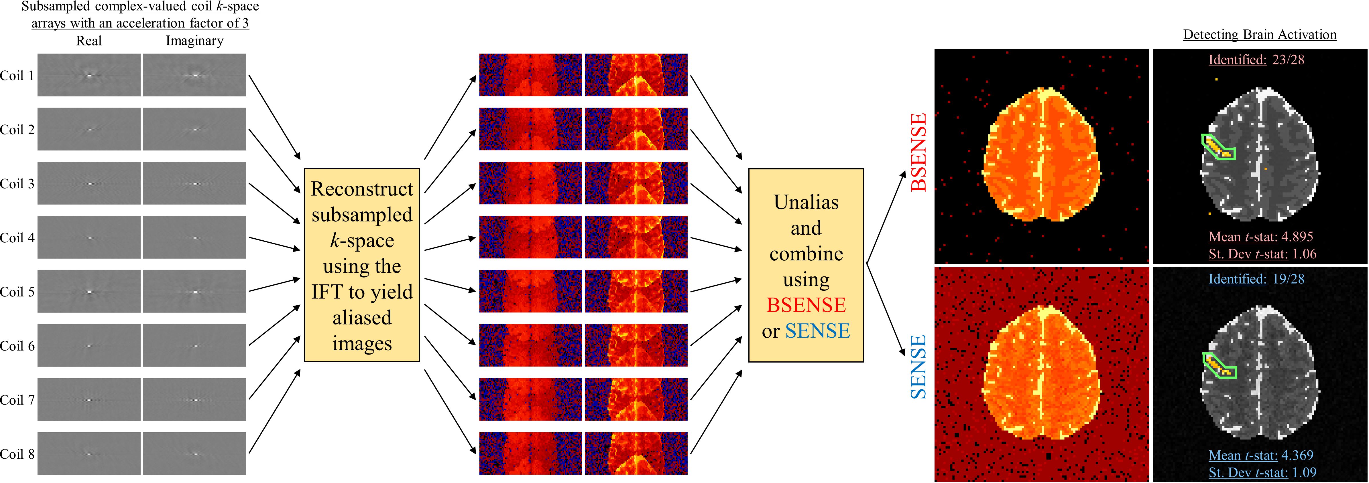
Functional MRI (fMRI) was developed in the early 1990’s as a technique to noninvasively observe the human brain in action. Measurements are arrays of complex-valued spatial frequencies, called k-space, which are approximately the Fourier transform of the image. The k-space arrays are reconstructed into images using an inverse Fourier transform (IFT). Measuring full arrays of data for all the slices that form the volume image takes a considerable amount of time. This limits the temporal and spatial resolution of the acquired images which can diminish effectively capturing brain activity. A solution for this is to measure less data by skipping lines in the spatial frequency arrays. This could allow for acquiring more images, obtaining higher resolution images, or simply reduce the overall scan time of the MRI process. In order to subsample k-space, multiple receiver coils are utilized in parallel to obtain a spatial frequency array which are reconstructed into coil-specific brain images. However, after applying the IFT to the subsampled k-space arrays, the images in each coil become aliased or appear as if they are "folded over." To obtain full field-of-view (FOV), the aliased coil images must be unfolded and combined to yield a full brain image. Common methods used in practice are SENSitvity Encoding (SENSE) and GeneRalized Autocalibrating Partial Parallel Acquisition (GRAPPA).

 Current Research

BSENSE - Bayesian SENSitivity Encoding

Traditional SENSE performs reconstruction via the relationship
    a_c^(ν) = S_c^(ν) v_c^(ν) + ε_c^(ν), ν = 1, ..., L
where a_c is the observed complex-valued aliased coil measurements, S_c is the matrix of unobserved complex-valued coil sensitivities, v_c is the unobserved complex-valued unaliased voxel values, ε_c is the additive complex-valued noise, and L is the total number of voxels in the full image divided by the acceleration factor yielding the total number of voxels in the aliased image. Prior to an fMRI experiment, a short non-task based set of full k-space volume arrays for each coil can be obtained and inverse Fourier transformed into full pre-scan coil calibration images. With an estimate of the complex-valued coil sensitivities Ŝ_c from these pre-scan calibration images, a least squares estimator of v_c for each voxel is given by
    v_c^(ν) = (Ŝ_c^(ν)H Ŝ_c^(ν))^-1 Ŝ_c^(ν)H a_c^(ν), ν = 1, ..., L
The Ŝ_c estimated from the pre-scan calibration images is then treated as a "known" parameter and is fixed at every time point in the fMRI time series. Since the design matrix S_c is generally ill-conditioned, the final reconstructed image can have degraded signal-to-noise ratio (SNR), or contain aliasing artifacts. Common approaches to mitigate this is the use of a regularizer which still introduces bias yielding a blurred image or can be computationally expensive. This motivates the use of a Bayesian approach to SENSE image reconstruction.
For the Bayesian approach, the unaliased voxels v, the coil sensitivities S, and the noise variance σ² are unobserved parameters that are specified with prior distributions. Combined with the data likelihood, we can formulate a conjugate, joint posterior distribution. Using all available information from the pre-scan calibration images, the priors are quantified for each unobserved parameter and assess other hyperparameters utilized for parameter estimation. Using the posterior distribution, two techniques are applied for estimating the unaliased voxels v, the coil sensitivities S, and the noise variance σ²: Maximum a posteriori (MAP) estimation using the Iterated Conditional Modes (ICM) optimization algorithm to find the joint posterior mode, and marginal posterior mean estimation via Gibbs sampling.




 

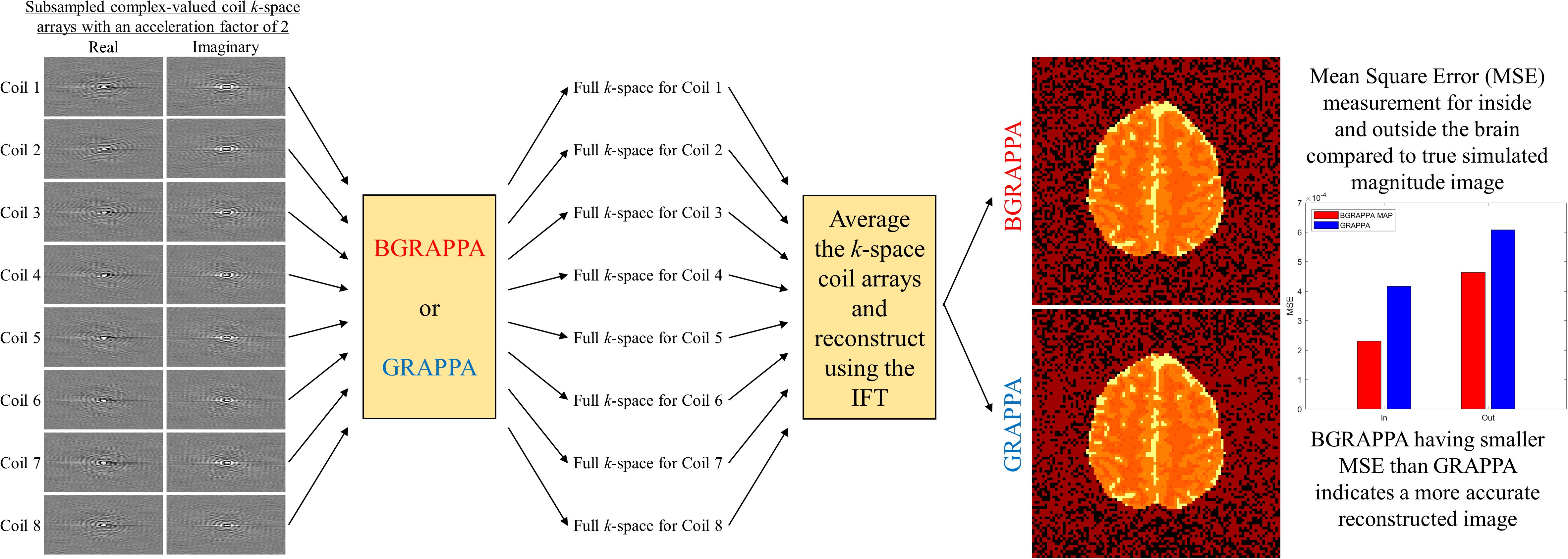
BGRAPPA - Bayesian GeneRalized Autocalibrating Partial Parallel Acquisition

GeneRalized Autocalibrating Partial Parallel Acquisition (GRAPPA) is a parallel imaging technique that yields full images from subsampled arrays of k-space. Unlike SENSE, GRAPPA operates in the spatial frequency domain. Before using the IFT, GRAPPA estimates the unobserved spatial frequencies, yielding full k-space arrays for each coil. The full k-space arrays are averaged and then inverse Fourier transformed into a single, full FOV brain image. GRAPPA uses localized weights to fill in the missing spatial frequencies of the subsampled k-space. The localized weights are assessed from pre-scan full coil calibration k-space. The model for the full calibration k-space arrays is
    f_calib^(κ) = w^(κ) f_a^(κ) + η^(κ), κ = 1, ..., K
where f_calib is the observed complex-valued calibration coil spatial frequencies, w is the matrix of unobserved localized weights, f_a is the complex-valued spatial frequencies located in the lines of k-space that will be observed in the fMRI experiment, η is the additive complex-valued noise, and K is the total number of spatial frequencies in the full k-space array divided by the acceleration factor yielding the total number of frequencies in the subsampled k-space. The localized weights are assessed using a least squares estimator
    w^(κ) = f_calib^(κ) f_a^(κ)H (f_a^(κ) f_a^(κ)H)^-1, κ = 1, ..., K
These localized weights are utilized to estimate the unobserved spatial frequencies at each point in the fMRI time series using the linear regression
    f_e^(κ) = w^(κ) f_p^(κ) + η^(κ), κ = 1, ..., K
where f_e is the estimated complex-valued missing spatial frequencies, w is the matrix of estimated localized weights, and f_p is the complex-valued observed spatial frequencies, η is the additive complex-valued noise. GRAPPA does have drawbacks such as storing and using potentially large matrices that would substantially increase reconstruction time or produce low-quality reconstructed images that would require further corrections. GRAPPA also discards valuable information from the calibration k-space arrays that can be used in estimating the unobserved spatial frequencies.
Due to these drawbacks, we introduce a Bayesian technique to GRAPPA (BGRAPPA) that incorporates all valuable prior information to estimate the unobserved k-space values. For the Bayesian technique, the GRAPPA linear regression is utilzied, but the parameters are treated differently. For BGRAPPA, f_e is the observed spatial frequencies, w is the matrix of estimated localized weights, and f_p is the estimated complex-valued missing spatial frequencies. The localized weights w, the unobserved spatial frequencies f_p, and the noise variance τ² from η ~ N(0,τ²I_nC) are unobserved parameters that are specified with prior distributions. Combined with the data likelihood, we can formulate a conjugate, joint posterior distribution. Using all available information from the pre-scan calibration spatial frequency arrays, the priors are quantified for each unobserved parameter and assess other hyperparameters utilized for parameter estimation. The two techniques applied for estimating the localized weights w, the unobserved spatial frequencies f_p, and the noise variance τ² are MAP estimation using the ICM optimization algorithm and the marginal posterior mean estimation via Gibbs sampling.